As a continuation of TensorFlow Flowers there is a cool tutorial on classifying Clothes using Keras, a high-level API to build and train deep learning models. It’s used for fast prototyping, advanced research, and production.
Prerequisites:
I am currently using Docker for the TensorFlow environment. If you are not familiar with Docker or have not read my post on Docker, I suggest you read that first
To start run the TensorFlow Docker Container with Jupyter notebook capabilities:
docker run -it -u 501 --rm -p 8888:8888 tensorflow/tensorflow:latest-py3-jupyter
Once the container is running you should see
To access the notebook, open this file in a browser: file:///.local/share/jupyter/runtime/nbserver-13-open.html Or copy and paste one of these URLs: http://(ace0315e3bc7 or 127.0.0.1):8888/?token=12iu8ods87asjdhha80d
So all you need to do is go into a browser and enter the url:
127.0.0.1:8888/?token=12iu8ods87asjdhha80d
Your Token will be different
If everything worked you should see a Jupyter Notebook
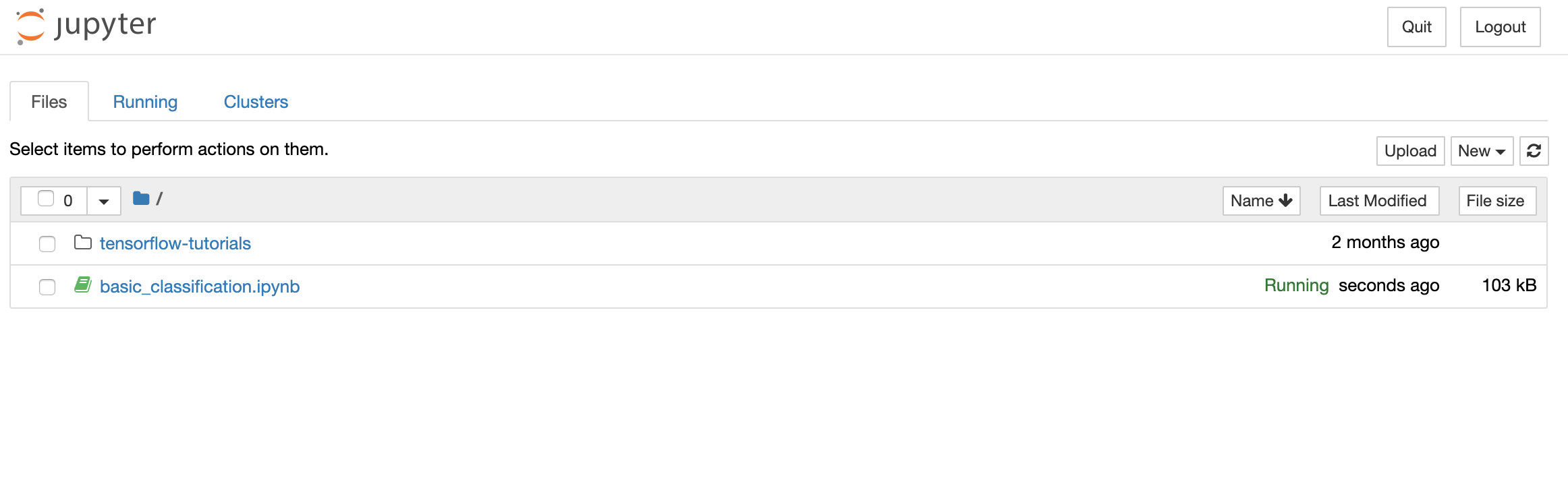 From there we will be using the “basic_classification.ipynb” notebook in the “tensorflow-tutorials” tutorials folder.
My thoughts on the module:
This tutorial uses TensorFlow 2.0 which is an upgrade from when I used 1.x in TensorFlow flowers so there were a few things I needed to get used to. Kera’s is now the default implemented neural network library instead of sklearn so I needed to understand the syntax. TensorFlow is starting to take more of a collaboration approach using codelabs which is a Jupyter notebook environment that requires no setup and runs entirely in the cloud. Its pretty cool and basically makes it so you don’t need to run Docker or setup any code environment locally. Everything saves to a cloud and collaborated on simultaneously. I will definitely be using in the future for more research I do.
Anyway, after getting over the hurdle of the changes to TensorFlow 2.0 I was able to get into the nitty gritty of the module. The goal is to train a neural network model to classify images of clothing, like sneakers and shirts. The hardest part was working with Kera’s because I have never seen it before. I will get into more depth on specifically what Kera’s is capable of later.
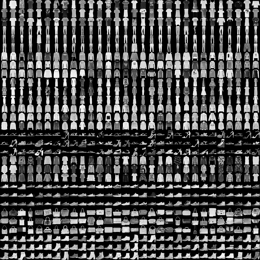
The first step after importing our libraries was to import the Fashion MNIST dataset. This is basically a replacement to the original MNIST used for handwriting classification. Originally I planned on doing handwritten classification but decided to go with the clothes classification because it seemed a little more challenging. I will most likely attempt the handwritten tutorial at another date for learning purposes.
fashion_mnist = keras.datasets.fashion_mnist

(train_images, train_labels), (test_images, test_labels) = fashion_mnist.load_data()
Loading the dataset return 4 arrays. 2 for training and 2 for testing. 1 for the actual images and 1 for the labels. As we learned before the labels are the output. Features are INPUT to a Classifier and LABEL is OUTPUT returned. In this case its a simple 0-9 array where each matches up to an article of clothing.
The raw data needs to be scrubbed and setup for the neural network to learn from. The module follows a really intuitive theme of showing visuals to help with understanding what is happening
plt.figure()
plt.imshow(train_images[5])
plt.colorbar()
plt.grid(False)
plt.show()
plt is matplotlib.pyplot imported from before and that allows us to visualize the pixel values of each article of clothing. The images look really accurate to the originals as sort of a heatmap of data.
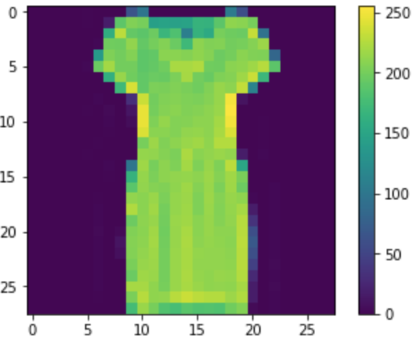
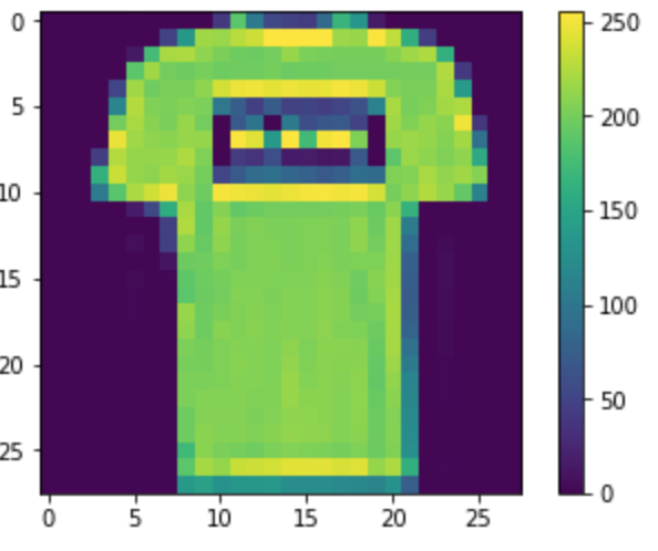
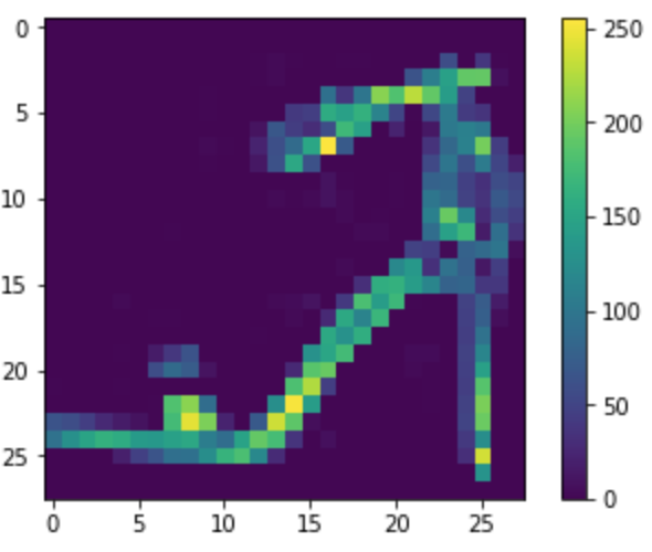
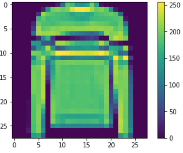
The actual act of scrubbing the data is pretty simple. The heatmap shows the pixel value up to 255. 0 being while and 255 being black. In order to properly use the data to train it needs to be a number 0 - 1 so all we need to do is pixel/255. From what I’ve learned these steps are critical to a good network. Without proper training data the model will never learn properly.
From there we can finally start building the model. Kera’s is used to make things immensely easier here. It’s a really high-level API and eventually I would like to dive deeper to see how exactly it works but for the purpose of this study I wanted to try and absorb as much as I could and not waste time on the nitty gritty.
model = keras.Sequential([
    keras.layers.Flatten(input_shape=(28, 28)),
    keras.layers.Dense(128, activation=tf.nn.relu),
    keras.layers.Dense(10, activation=tf.nn.softmax)
])
Kera’s Flatten will take the 28 by 28 images and make them 1-d array of784 pixels. Kera’s Dense is the neural network we are familiar with from prior lessons. It creates one network with 128 neurons and the other with 10. The 10 is a probability of certainty of the article of clothing.
After the model is made, we test and train the data. Since the data is given for a tutorial the training and testing is pretty intuitive and does what you would expect. Trains on the images then tests a few for accuracy. I was able to get .89 after 5 epochs of training. Then when I tested the model on new data it dropped to .86. Reason being was Overfitting.
It turns out, the accuracy on the test dataset is a little less than the accuracy on the training dataset. This gap between training accuracy and test accuracy is an example of overfitting. Overfitting is when a machine learning model performs worse on new data than on their training data.
This is a concept I have heard a lot about since the beginning of this study but never actually saw it happen with data. It was cool to see how Overfitting can make a learning model perform worse and how important testing it. I found a research paper by a few researches in the University of Toronto on overfitting and how to prevent it using dropout. In the paper they describe Dropout as
“randomly dropping units (along with their connections) from the neural network during training. This prevents units from co-adapting too much. During training, dropout samples from an exponential number of different “thinned” networks. At test time, it is easy to approximate the effect of averaging the predictions of all these thinned networks by simply using a single untinned network that has smaller weights.” (Srivastava, Hinton, Krizhevsky, Sutskever, & Salakhutdinov 2014).
It would be cool to test this theory at a later date with this data and see if accuracy increases.
Finally, after training the model and testing it was successfully able to make predictions on clothing with high accuracy
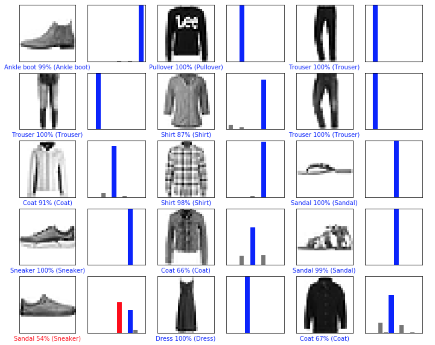
The blue lines vs red lines indication right and wrong predictions and the line corresponds to the 0-9 label output we configured earlier.
All in all the module was a nice introduction to TensorFlow 2.0 and I think the project is doing great things for collaborating with others on research. Learning more about Kera’s is definitely something on my to-do list. The TensorFlow 2.0 tutorials has a lot of really cool tutorials setup that I will continue to explore even after the independent study is over.
Sources
Dietterich, Tom. “Overfitting and Undercomputing in Machine Learning.” ACM Computing Surveys (CSUR), vol. 27, no. 3, 1995, pp. 326-327.
Srivastava, Nitish, et al. Dropout: a Simple Way to Prevent Neural Networks from Overfitting. The Journal of Machine Learning Research, 2014.
http://yann.lecun.com/exdb/mnist/
colab.research.google.com